Equity curve feedback, or equity curve filter, uses the equity curve of a trading system to determine when to take trades from that system and when to just watch them.
The calculation begins with a trading system. Call this the “base” system. In the example below, it is a moving average crossover. When one moving average crosses the other, a Buy or Sell signal is generated.
Use of the equity curve is done in two steps.
1. Keep track of all of the trades that are signaled, and the equity curve produced by these trades. Call these the “shadow” trades and the “shadow” equity curve.
2. Apply some technical analysis technique to the shadow equity curve as if that is a price series. When the results of “trading” the equity curve are good, take the signals generated by the base system. When they are poor, remain flat.
Trading the equity curve is essentially the same as trading a price series. Apply any indicator you want to the daily equity. In the example below, the equity curve is defined to be “good” when it is above its moving average, and “poor” when below. When it is good, signals from the basic system are passed through; when it is poor, all signals are blocked.
If you are running a trading system on a watchlist, the equity curve filter is applied to each individual issue before the results are gathered into the portfolio.
When evaluating use of an equity curve filter, the process is essentially the same as applying a trading system to a stock. If the stock tends to trend well, the type of trading system that will be profitable is trend-following. If the stock spends more time in a trading range and oscillating, the type of trading system that will be profitable is mean-reverting. The length of time a typical position is held makes a difference.
The same principle applies to the equity curve.
If winning trades tend to be followed by winning trades and losing trades followed by losing trades, then the type of equity curve filter that will be helpful is a trend-following equity curve filter. For example, a moving average applied to daily equity, allowing trades when the equity is above its moving average and blocking trades when it is below.
If winning trades tend to be followed by losing trades and losing trades followed by winning trades, then the type of equity curve filter that will be helpful is a mean-reverting equity curve filter. For example, an oscillator based on the RSI of the equity, allowing trades at low values and blocking trades at high values.
In the code posted, the equity curve filter is being used to evaluate daily equity and either allow or block new trades. It can also be used to exit existing trades before the trading system causes the exit. To do this, incorporate some calculation on the “e” variable as a component of the “Sell” command. For example, Sell = Sell OR ROC(e,5)<0;
Over All ---- The important logic is that built in to your trading system's entries and exits (and position size and risk control).
Do not expect an equity curve filter to rescue the performance of an ailing trading system.
--------------------------------------------
Here is the AmiBroker code
///////////////////////////////////////////
//    EquityCurveFeedback.afl
//
//    Howard Bandy
//    November 2011
//
//    There are many ways to use the equity
//    in the trading account, and its variation,
//    to act as a filter to allow or block trades.
//
//    This code shows one example of applying
//    trading system logic to the equity curve
//    created by another trading system.
//
//    The first system is a simple moving
//    average crossover — it could be any system.
//
MALength1 = 5; //Optimize(“MALength1?,5,2,50,2);
MALength2 = 1; //Optimize(“MALength2?,1,1,51,2);

Buy = Cross( MA( C, MALength1 ), MA( C, MALength2 ) );
Sell = Cross( MA( C, MALength2 ), MA( C, MALength1 ) );

Buy = ExRem( Buy, Sell );
Sell = ExRem( Sell, Buy );

e = Equity();

Plot( C, “C”, colorBlack, styleCandle );

//PlotShapes( Buy*shapeUpArrow + Sell*shapeDownArrow,
//            IIf( Buy, colorGreen, colorRed ) );
Plot( e, “Equity”, colorGreen, styleLine | styleLeftAxisScale );

//    The equity curve is choppy.
//    If there are positive serial correlations
//    between daily equity values, then we expect
//    up days to be followed generally by more up days,
//    and down days by more down days.
//    So we might try applying a trend following system
//    to the equity curve.
//    When the equity curve is above its moving average,
//    the system is working, and we should take trades.
//    When the equity curve is below its moving average,
//    the system is out-of-sync, and we should block trades.
//    EquityMALength is the lookback period for the equity
//    curve moving average.
//    We will set Pass to either 0 or 1.
//    Pass==0 blocks trades, Pass==1 allows trades.

EquityMALength = 6; //Optimize( “EquityMALength”, 6, 2, 20, 1 );
EquityMA = DEMA( e, EquityMALength );

Plot( EquityMA, “equityMA”, colorBrightGreen, styleLine | styleLeftAxisScale );

Pass = IIf( e >= EquityMA, 1, 0 );
Buy = Buy AND Ref(Pass,-1);

Buy = ExRem( Buy, Sell );
Sell = ExRem( Sell, Buy );

e1 = Equity();

Plot( e1, “FilteredEquity”, colorBlue, styleLine | styleLeftAxisScale );

///////////////////////// end ///////////////////////////
Here is a chart showing how it worked for XOM from 1998 through 2011.