Tradaingmarkets.com on option strategies
Címkék: trading options tradingmarkets.com
2015.01.11. 23:40
One of the most powerful aspects of trading with options is that there’s an option strategy for almost any situation. Today we’re going to introduce two of those strategies: straddles and strangles. Both straddles and strangles are non-directional strategies, meaning that they have the ability to profit whether the price of the underlying security moves up or down.
 A long straddle involves buying a call and a put on the same underlying security. Both options have the same expiration date and the same strike price. The risk profile for a long straddle is shown in the box to the left.
A risk profile, sometimes called a profit diagram, shows how much the option strategy will gain or lose based on the stock price at expiration. All long straddles have a risk profile shaped like a V, with the base of the V falling $C below the horizontal breakeven line, where $C is the total cost of entering the straddle. In terms of the stock price, the base of the V coincides with the strike used for the call and put. In other words, if buying a 125 strike straddle costs $7/share ($700/contract), then the maximum loss will occur if the stock expires at a price of exactly $125, making both options worthless at expiration.
The breakeven points for a long straddle fall $C above and below the strike price. Continuing the example from above, the stock price needs to be below $118 or above $132 at expiration for the straddle to be profitable. The further below $118 or above $132 the stock price is, the more profitable the straddle will be. Therefore, we can see that buying a long straddle is a bet that the stock price will move significantly by expiration.
 Not surprisingly, a short straddle is a bet that the stock price will not move significantly before expiration. A short straddle is created by selling (shorting) a call and a put with the same expiration date and the same strike price. The short straddle risk profile is shown in the box to the left. As with all short option strategies, the profit is capped at the amount of premium collected ($P) when the position was entered. With a short straddle, that occurs when the stock price is exactly at the strike price at expiration. If the stock moves more than $P above or below the strike, the position will incur losses, and those potential losses are theoretically unlimited.
Strangles are close cousins of straddles. The difference is that strangles are created by buying (long strangle) or selling (short strangle) a call and a put with the same expiration date and different strike prices. The risk profiles are shown below.


A long strangle is less expensive to establish than a long straddle, because it uses an out of the money (OTM) call and put, rather than the pricier at the money (ATM) options used by the strangle. The disadvantage of the strangle is that the stock price has to move further before the position becomes profitable. For a long straddle with a cost of $C, the lower breakeven point occurs when the stock price expires $C below the put strike, and the upper breakeven point is $C above the call strike. Once the stock price moves outside this range, there is unlimited profit potential.
Similarly, the short strangle garners a smaller premium (max profit) than the short straddle. However, you get to keep the entire premium ($P) as long as the stock price stays between the call and put strikes, so there’s a larger margin of error with short strangles as compared to short straddles. As with the long strangle, breakeven occurs $P below the put strike and $P above the call strike.
----------------------
In the previous article we introduced two non-directional option
strategies: straddles and strangles. We’ll now discuss when to use
these strategies, and how to evaluate their potential for success.
Long straddles and strangles are useful tools when you think that a stock
will undergo a large move, but you’re not sure whether the move will be
up or down. Short straddles and strangles are simply the opposite side
of this trade, and are essentially a bet that the stock price will not
change significantly before expiration.
Some traders like to use the long version of these strategies when a company is announcing
earnings or introducing a new product to the marketplace. However, it’s
always hard to know how much of the news is already “priced in”, i.e.
reflected in the current price of the stock. So how can we tell if the
change in stock price is likely to be large enough for a long straddle
or strangle to be profitable?
There are at least three ways to gauge our chances of success with a straddle or strangle:
- Use a quantified, back-tested strategy.Obviously this is our preferred method. Developing a well-defined
strategy with precise entry and exit rules and then back-testing that
strategy with reliable data across a variety of market conditions gives
us an excellent perspective of how the strategy has performed in the
past, and therefore provides some reasonable (though certainly not
infallible) expectations of how it will perform in the future.The
challenge here lies with the “reliable data” aspect of back-testing.
While there are many, many sources for high-quality historical stock and
ETF data, good options data is much more difficult to obtain. This is
partly due to its volume (consider that a single stock may have dozens
or even hundreds of strike prices for each of several active
expirations), and partly due to its transience (most traders don’t care
about the price of an option that expired three years ago). - Use stock prices as a proxy for option prices.If you don’t have access to option data, you may be able to gain some
insight by looking at historical stock prices. With AAPL earnings being
announced this week, you may have thought that last Friday would be a
good time to purchase a straddle using weekly options. However, the ATM
straddle had a price of around $36 on Friday, which is 7.2% of AAPL’s
$500 stock price. Recall that for a long straddle to be profitable, the
stock price needs to move up or down by more than the cost of the
straddle. Assuming you’d like to make at least a 10% profit on your
trade, you could check how many times AAPL has moved by 8% or more
during earnings week. Over the past three years, it’s happened 5 out of
12 times. Do you want to place $3600 on a bet that’s been a winner less
than 50% of the time in recent years? - Apply an option pricing model to current option dataThis is the most complicated of the three solutions, but is not as
intimidating as it sounds because your trading platform will do most of
the work for you.Theoretically, the price of an option is determined by a
number of factors. The four most influential ones are:- Price of the underlying stock
- Strike price of the option
- Time until expiration of the option contract
- Implied (expected) volatility of the stock price
The actual option price and all the values above except implied volatility
are easily obtained. Because we have all the other elements, we can
algebraically solve for implied volatility, which in turn allows us to
calculate delta (one of the option Greeks) and the probability that the
option will expire in the money (ITM). All platforms will have a way to
report delta and the other Greeks. Some platforms will also report the
probability of the option expiring ITM. For example, here was the weekly
option chain for AAPL as of Friday, January 18th, as shown on TD
Ameritrade’s thinkorswim platform. Calls are on the left, puts are on
the right, and strike prices are in the blue section in the middle.
Notice that the value of delta is quite close to “Prob ITM”, which is the
probability that the option will expire in the money. Therefore, delta
is a reasonable substitute for probability of expiring in the money if
your platform doesn’t provide the latter value.How does that help us? Well, we know that the 500 strike straddle would have cost just
--------------------------------------------------
under $36 last Friday. Therefore, to profit we need AAPL to move by more
than that amount, so let’s say we’d like at least a $40 move. The
current AAPL price of $500 plus a $40 move would be $540. Looking at the
option data above, we see that the 540 call has a 17.68% chance of
expiring in the money, i.e. there’s a 17.68% chance that the price of
AAPL will be above $540 by expiration. Similarly, the OTM option that is
$40 below the current stock price is the 460 put, which has an 18.49%
chance of expiring in the money. Therefore, the combined wisdom of the
marketplace, as encapsulated in the price of the options, is that
there’s less than a 20% chance that the price of AAPL will move
sufficiently to make the straddle profitable.
Obviously the market
is not always correct, and sometimes the market participants get
surprised. Would you be willing to bet your money that this is one of
those times?
The “Greeks” are a measure of the sensitivity of the option price to small changes in the main inputs to the pricing model: price, volatility, time (until expiration), and interest rate. Other than the mention of “Rho” below, I’m excluding interest from further discussion because at current rates it is largely irrelevant. These Greeks generally need to be calculated by some kind of modeling software.
Let’s now explore Delta, Gamma, Vega, Theta and Rho to gain a better understanding of some of the factors influencing option pricing.
Delta:
Delta tells us how much the option price is expected to move compared to the underlying security, generating a positive value for calls and a negative one for puts. It is usually expressed as a decimal (eg .75), sometimes expressed as a stock equivalent (eg .75 * 100 shares = 75 deltas). So a .75 delta call would move approximately .75 for a 1.00 up-move in the underlying, -.75 for a 1.00 down-move. I say approximately because delta is not static, it changes with price movement (see “Gamma”) as well as with changes in volatility and time.
At this point some general observations about delta can be made:
- At-the-money (“ATM”) options are about +/- .50.
- The deeper in-the-money (“ITM”), the more the options approach +/- 1.00.
- The further out-of-the-money (“OTM”), the more the options approach +/- .00.
Nearer term ITM options have larger absolute value delta than a same strike further term. Near term OTM options have smaller absolute value delta than further term. The lower the volatility, the faster options approach +/- 0.00/1.00 as they move away from ATM; the higher the volatility, the more all options approach +/- .50.
Gamma:
Delta is so important among the Greeks that it actually has its own Greek – Gamma. Gamma measures how fast the delta changes with stock price movement. ATM options have the largest gamma, while gamma declines as the option moves away from ATM. Nearer term options have more gamma than the same strike price further term option. One way to remember this is to think about an ATM option one trade away from expiring, a one tick move either way changes it to 0.00/1.00 delta.
Vega:
Vega gives us an idea of how much the option price would move with a 1% change in volatility. This has more use in trading options against other options than in using options as a stock equivalent. ATM options will have the most vega, and vega will decrease as the options move in or out of the money. For the same strike price, further term options will have more vega. Please note that the volatility used here is not historic (or statistical) volatility which is an exact number based on price history, but rather a forecast volatility, the marketplace’s best guess as to the future volatility. “Implied volatility” is calculated by using the option price as an input to the model and returning the volatility that implies.
Theta:
Theta is a measure of how much the option price loses in 1 day. Its value can be approximated as the extrinsic value (essentially vega) divided by the number of days until expiration. So ATM options decay the most. Nearer term options decay faster, with the number of days being a more important factor than the extrinsic value.
Rho:
Rho indicates how much the option price will change with a 1% change in interest rate. For now, this is just something to keep in the back of your mind, and revisit if/when interest rates become relevant again in the future.
It’s important to note that the greeks are additive in nature. When I say additive I mean that the total delta exposure for all the options on an underlying vehicle can be found by adding the delta of each individual option. In looking at the core simplified level, we see that a positive greek value means that the options price benefits from an up-move in that specific model input, while the opposite is true as well for a negative value.
For our purposes, we will be using options as a stock equivalent, so the most important Greeks are delta and theta. Delta establishes our expectations for absolute return relative to the stock and gives us a value that we can use to calculate how much leverage we need to achieve equal market exposure as the underlying stock. Theta tells us how much we are paying (for long options) or collecting (for short options) in whatever strategy we are using for a stock equivalent. This directly connects us to the next topic we’ll be covering in our series; join us next time as we cover the basic options trading strategies and their characteristics.
---------------------------------------
Before we dive into the basic stock replacement strategies, I want to explain how to determine net contracts for a single underlying stock, both on the long side and the short side. The bottom line is that if you are net long contracts you have unlimited reward and limited risk, if you are net short contracts you have limited reward and unlimited risk (I’m considering a short put to have unlimited risk, although technically it is limited to stock price – option price). Limited risk doesn’t mean insignificant risk, but rather risk that can be exactly quantified, therefore exactly controlled.
On the long side, you simply add all the call positions (keeping their signs) and also +/- 1 call for every +/- 100 shares of stock. On the short side, you add all the put positions and also +/- 1 put for every -/+ 100 shares of stock (short stock yields long puts). If the net contracts happen to come to zero, you have limited reward and limited risk. We’re going to examine 3 basic strategies on the long side: long call, short put, and long call spread (with mention of equivalent positions).
Once you understand these, it is easy to see that the equivalent short strategies mirror the long strategies — a table below will show how the characteristics are related.
Long Calls
A long call is the most basic bullish strategy. It is characterized by unlimited reward (to the upside) and limited risk (to the downside). This comes at a price, which is the premium over parity that is paid. That premium erodes on the way to the expiration date (especially in the last week), and hopefully the premium is replaced by increased intrinsic value. For maximum success, you have to be right on both price and time. The impact of time decay is often underappreciated and too early an expiration is chosen. Assuming you have a back-tested equity strategy, you should have an idea of how long the trade should take on average, and the likely maximum (even more definitive if you happen to use a time stop). I would suggest that you pick an expiration far enough away that the average trade exits at least a week before expiration, and even consider an expiration far enough away so the maximum time in the trade exits similarly.
The next consideration is what strike to use. If you have some technical reason (e.g. support, 200MA) to use a particular price, your decision is already made. Otherwise, if you are going to take a conservative approach and trade 1 contract for every 100 shares you would normally trade, in-the-money options will probably be the way to go. This way you’ll get closer to the same market exposure.
Below are P&L graphs for an ITM, ATM, and OTM call (all graphs are based on a theoretical stock trading at 100, .16 implied volatility, 20 trading days until expiration, ITM=98, ATM=100, OTM=102):
Long Call ITM:

Long Call ATM:

Long Call OTM:

You might notice that the time decay lost over the first 5 days is less than over the next 5 days, and so on. Also, it is worth noting that a 2% move up over 10 days is essentially breakeven for the OTM call.
Short Puts
A short put is an alternative bullish strategy and is the equivalent of a covered call. This strategy has limited reward and unlimited risk. In return for assuming the call buyer’s risk, the put seller collects any premium erosion that results. Since decay happens fastest at the end of an option’s lifetime, a shorter expiration is desired. You still want to leave enough time for the trade to play out; otherwise you get mired in what to do when the short option expires. The strike price considerations are similar, if you have technical reasons to use a certain price, by all means do so. Otherwise, ITM puts give the most market exposure, offering the opportunity to capture the premium over parity and hopefully some or all of the intrinsic value. Because of the unlimited risk, to sell more than 1 put for every 100 shares you would normally buy is very aggressive, and thereby multiplying your risk. P&L graphs follow below:
Short Put ITM:

Short Put ATM:

Short Put OTM

One interesting aspect of selling versus buying is that you no longer need to be right, just not to be wrong.
Bull Spreads
A blended approach is to buy a call spread (or sell a put spread, the risk characteristics are the same), that is, buy one strike price and sell a higher strike price. Since a spread is contract neutral, there is limited reward and limited risk. Assuming the long and short contracts are equidistant from the stock price, there is no or very little time decay. As the stock price gets nearer to one side, the spread starts to favor the characteristics of that side, although to a lesser extent than that side by itself. With a short contract in the mix, you can afford to pick a closer expiration with the proviso that you would like the trade to be exited before expiration. If technical considerations exist for the strike prices – use those – otherwise you can use the same considerations for long call for the lower strike, and I suggest a higher strike that at least covers the extrinsic value in the long call. P&L graphs follow:
Bull Spread ITM:

Bull Spread ATM:

Bull Spread OTM

The ITM (98-100) and OTM (100-102) spreads are 2 dollars wide, the ATM (98-102) 4 dollars wide. One thing you may notice is that the long call spread develops more slowly than the other strategies, just something to be aware of if you choose this strategy. It’s also important to mention that the transaction costs (commissions, bid-ask spread) are doubled in this case.

*Technically limited to Stock Price – Option Price, but relatively unlimited
**Will take on characteristics of option closest to stock price
This summarizes the long strategies we have discussed and includes the mirrored short strategies.
Another consideration to keep in mind is that volatility can be thought of as measuring fear, thus if the market is moving up, volatility tends to decrease (and vice-versa). So a successful long call is going to be negatively impacted by the change in volatility, while a successful short put will gain. This tendency of volatility to move with the market is why the conventional wisdom is to sell puts for a move up and to buy puts for a move down, in a way it’s like having the wind at your back. This phenomenon is also favorable for a bull spread (with a long ITM call) bought on a dip — the implied volatility is likely relatively high and will decrease on an ensuing up-move.
Considerations in trading a spread:
If your software/broker permits trading the spread as a spread, by all means do so. If you have time to work it, you can probably start near using the midpoints of each bid-ask and work from there, otherwise use a market order. If you have to leg into it, you generally want to do the side with the widest bid-ask first. It may be possible to bid/offer one side with the idea of then hitting the bid/taking the offer of the other side, but many brokerages charge cancellation fees (sometimes even if the exchanges themselves don’t), so be careful when attempting that.
I said before that buying a call spread is equivalent to selling a put spread (with the same strike prices). So how do you decide which to do? Generally, the bid-ask spread will determine that. You want the smaller spreads, and that will generally come with the smaller-priced options.
------------------------------------------------
After defining and detailing the fundamentals of options trading, we can move ahead with comparing and contrasting trading results. We’ll now take a look at what could have happened if we used options in place of SPY stock, using a strategy loosely based on the one Larry Connors presented in his preview of the upcoming Quantified Options Trading Strategies Summit 2013:
- Entry: SPY 2-period RSI < 5
- Exit: SPY 2-period RSI > 70
There were 3 consecutive trades starting in late July 2011 that should prove illustrative and will be covered throughout the next 3 installments of this series- a loser, a winner, and a break-even trade if SPY stock were traded. Since the strategy was based on the SPY 4PM EST close, I simulated option prices for 3 strikes with the Black-Scholes model, inputting that day’s implied volatility (IV) for the middle (ATM) strike, 4% higher IV for the lower (ITM) strike and 4% lower IV for the higher (OTM) strike. This should give us a reasonable approximation of comparative results.
The first trade we’ll look at had an entry on July 27, 2011 and didn’t exit until Aug. 15, 2011.

Anyone who was trading mean-reversion strategies at that time will remember that period all too well. The results based on using Aug. 2011 monthly options are shown below (no commissions/slippage):

The first group of results reflects using 1 option contract as a replacement for 100 shares of SPY. The long calls had a smaller loss in dollars although in percentage terms took a 100% loss. This should reinforce the notion that a 100% loss is a very real possibility when trading options. The short puts lost much more than the long calls. Essentially they did better than long SPY because of the premium collected, where a covered call would have given the same results. The bull spreads, even the $4 spread, fared the best. This can be attributed to the much lower market and dollar exposure (if you compare the deltas on the spreads vs. the single options). Also, notice that there was no real difference between the long call (debit) spread vs. the short put (credit) spread.

The second group of results shows what happens if you increase the contracts so that the market exposure is equivalent to SPY stock.
Number of contracts * Deltas = SPY equivalents
Long calls continue to lose less than SPY stock. Short puts do worse, since as the trade goes bad the market exposure gets bigger. The bull spreads perform in between, not surprising considering their long/short options structure. What is somewhat alarming is how many $2 spreads were needed to establish the same market exposure as SPY stock — commissions and liquidity would certainly become a factor.
Most of these results show reduced losses in what was a very bad trade, so using options would have been preferable. In the next installment of the series we’ll look at a winning trade and see if the same impression is true there as well.
-------------------------------------------------
In the first comparative look at our model trades from late Jul 2011 the data proved that an options trade would have yielded better results than the SPY stock on its own. Now we’ll look at the 2nd, and this time a winning trade, to see how using options would have compared to using the underlying SPY stock. This trade entered on Sep. 22, 2011 and exited 3 days later on Sep. 27, 2011.

The results from using Oct. 2011 monthly options are shown below (no commissions/slippage):

These results once again reflect using 1 option contract as a replacement for 100 shares of SPY. The long calls/short puts made about 50% of what the SPY trade made. This was a good scenario for long calls, a relatively sharp move in a short period of time. The short puts managed to keep pace and would have outperformed the long calls if the move had taken longer and/or the implied volatility had gone down significantly. The bull spreads didn’t do so well, this just emphasizes that they are slower in developing profits.

We now see what happens if the market exposure is increased to that of the SPY trade. The long calls have done very nicely, coming close to the SPY performance. The short puts have done even better than the calls or SPY, something to be hoped for considering their considerable amount of extra risk (remember how they fared in the first trade). Once again, the bull spreads end up roughly equivalent to SPY, in between long calls and short puts.
So far the options have looked pretty good compared to SPY, but both of these trades should have favored options.
For the next and last trade we will be analyzing one that was break-even for SPY. In the final installment to our options trading series, we’ll see how using options would have worked out once again and wrap up the topics we have covered so far throughout the course of this options primer.
-------------------------------------------
In this final installment of How to Trade Options we’ll look at a break-even trade and analyze the results, and then touch on what we’ve learned to reiterate the key things you should take away from the series. Our final trade entered on Nov. 21, 2011 and exited 4 trading days later on Nov. 28, 2011.

This was essentially a break-even trade if using SPY stock. Below we see the results if Dec. 2011 monthly options had been used instead:

These results once again reflect using 1 option contract as a replacement for 100 shares of SPY. The results are mixed. The long calls have lost money, suffering from time decay. The short puts have made money, collecting the time decay (an example of not being wrong). The bull spreads have done a little worse than SPY stock, but still essentially break-even, again in between long calls and short puts.

If the market exposure is increased to that of the SPY trade, the results are similar, just bigger because of the extra contracts.
The first two trades showed the use of options at their best, avoiding a very large loss on a very bad trade, and participating significantly on a quick sharp move up. The last trade was an example of when using options was a bad choice (in hindsight that is). Most options trades will have results somewhere in-between the examples.
Each of the 3 basic strategies has a best/worst scenario relative to trading SPY stock:
- The long call’s best scenario is an immediate sharp move up, while the worst scenario is a slow grind to the strike price.
- The short put’s best is a slow grind to the strike price, while the worst is an immediate sharp move down.
- The bull spread does best with a slow grind to the short option strike price, while the worst is a slow grind to the long option strike price.
If you’ve already been trading options and use only one of the 3 basic strategies presented, you might consider when to use one of the others. If you normally buy calls, but find the implied volatility (premium) too high, you could sell a higher strike call and try a bull spread instead, or sell a naked put. If you normally sell puts, but you think the implied volatility is too low, you could buy calls or do a bull spread instead. If your M.O. is to put on bull spreads, but you think you’re not getting enough for the short option, maybe trading long calls becomes appropriate.
With all these complicated choices, why even bother with using options instead? One reason is for risk control, taking advantage of limited risk to help smooth the equity curve. Another, more subtle reason is to take advantage of the leverage to allow for participation in an infrequent trade opportunity without tying up capital during idle periods. For instance, let’s say you trade equities on a swing basis, but also use a strategy like we were using in the examples — a strategy that triggers once a month on average. Instead of keeping a large amount of cash on the sidelines waiting for the infrequent trade, you could decide ahead of time how much you were willing to lose when that trade came around and keep that amount of cash available instead to buy calls, and free up the rest for the swing trades.
We can’t leave without at least a brief discussion of ITM, ATM, or OTM options.
Deep ITM options are basically stock, although still affording some limited risk and reduced capital use. Far OTM options are often called lottery tickets, they are almost always 100% losers, and their payoff comes with an extremely large and immediate move (something like a takeover — hard to imagine a SPY takeover).
I’d suggest that options between 70 and 30 deltas are more what we are considering. I will point out that if an OTM call makes money, then so will an ATM or ITM. Likewise if an ATM call makes money, so will the ITM. The same cannot be said in reverse, if an ITM is profitable, the others may or may not be profitable. On the other hand, if an ITM call loses, so will the ATM and ITM; if an ATM call loses, so will the OTM. The reverse is not true, if an OTM is unprofitable, that doesn’t mean the ATM and ITM is also unprofitable. If the same number of contracts is being used, ITM clearly has the advantage, a higher chance of success, and a higher amount of profit if right, but a larger loss exposure. If different number of contracts are used (either based on deltas or option price), while it is possible for the OTM to have a higher amount of profit (on a very large move), the ITM will always have a higher chance of success and will always be profitable–if any are profitable.
Let’s review what has been presented throughout this series.
- We defined calls and puts, and identified the factors that go into determining an option’s price.
- We showed the relationship between stock, call, and put and showed how each can be expressed in terms of the others.
- We defined the Greeks, the language used to talk about and to measure the pricing factors.
- We identified three basic strategies to use options as a replacement for stock and graphically showed how the P&L developed through expiration.
- We then showed how the three strategies would have compared to using stock across three extremes of trades to get an idea of what to expect.
- We briefly explored the best and worse scenarios for each strategy.
- Finally, we talked about how using options for infrequent trades allows participation while freeing capital for trades that happen more often.
Maybe the most important point made was that options do not eliminate risk, they just redistribute it. If you buy calls for the downside protection, you give up some of the upside, and lose on sideways action. If you short puts for the premium, you cap the upside, get only limited protection to the downside, and gain if very little happens. If you put on bull spreads, you cap both the downside and the upside, and have less market exposure that takes longer to mature.
Whatever you choose to do, you should now have an idea of what to expect. It is fine to be disappointed or pleased with the outcome, but you shouldn’t be surprised.
Ajánlott bejegyzések:
A bejegyzés trackback címe:
Kommentek:
A hozzászólások a vonatkozó jogszabályok értelmében felhasználói tartalomnak minősülnek, értük a szolgáltatás technikai üzemeltetője semmilyen felelősséget nem vállal, azokat nem ellenőrzi. Kifogás esetén forduljon a blog szerkesztőjéhez. Részletek a Felhasználási feltételekben és az adatvédelmi tájékoztatóban.